The Rasch chapter built one item response model from scratch and promised there was a wider world. Here it is. Item Response Theory (IRT) is a whole family of models for the same task - measuring people from their item responses - and generalizability theory (G-theory) is a broad extension of reliability that asks not only “how much error?” but “error from what?” Both are areas where the authors have published extensively, often together in a single study.
24.1 Learning Objectives
See how the 2-parameter (2PL) model generalizes Rasch by letting items differ in discrimination.
Read an item characteristic curve and know what its slope and location mean.
Decompose measurement error into facets with generalizability theory.
Compute a G-coefficient and use a D-study to design a measure - the “how many items?” question.
24.2 Beyond Rasch: Items That Discriminate Differently
Rasch makes a strong, simple assumption: every item is equally good at separating people; items differ only in difficulty. The 2PL model relaxes it, giving each item its own discrimination\(a_i\) (how sharply it distinguishes high from low) alongside its difficulty \(b_i\):
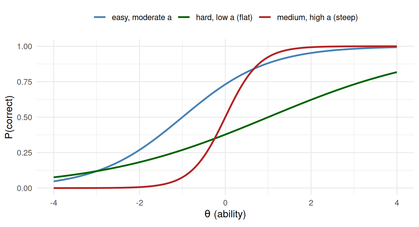
The clearest way to feel the difference is to look at the items. An item’s characteristic curve plots the probability of a correct/endorsed response against ability \(\theta\). Difficulty slides the curve left-right; discrimination changes its steepness:
library(tidyverse) # dplyr, ggplot2, purrr, tibble, readr, stringr, forcatslibrary(broom) # tidy(), glance(), augment() for model outputsource("_common.R") # book-wide helpers: round2(), fmt_p(), tidy2()icc <-function(theta, a, b) 1/ (1+exp(-a * (theta - b))) # 2PL curveitems <-tibble(item =c("easy, moderate a", "medium, high a (steep)", "hard, low a (flat)"),a =c(1.0, 2.5, 0.5), # discrimination (steepness)b =c(-1, 0.0, 1.0) # difficulty (left-right location))crossing(theta =seq(-4, 4, length.out =300), items) |>mutate(p =icc(theta, a, b)) |>ggplot(aes(x = theta, y = p, colour = item)) +geom_line(linewidth =1) +scale_colour_manual(name =NULL,values =c("easy, moderate a"="steelblue","medium, high a (steep)"="firebrick","hard, low a (flat)"="darkgreen") ) +coord_cartesian(ylim =c(0, 1)) +labs(x =expression(theta ~"(ability)"), y ="P(correct)") +theme_book() +theme(legend.position ="top")
The steep red item is discriminating: over a narrow band of ability it flips from “probably wrong” to “probably right,” so it sorts people sharply there. The flat green item barely distinguishes anyone - its responses are nearly a coin flip across a wide ability range. Rasch is the special case where every curve has the same slope; the 2PL, and its polytomous cousin the Graded Response Model (which we met dissecting depression profiles), let the data say otherwise. In practice you fit these with a maintained engine:
library(mirt) # shown, not run on the book's serverfit <-mirt(data, 1, itemtype ="2PL") # or "graded" for 0..k items (GRM)coef(fit, simplify =TRUE) # each item's discrimination (a) and difficulty (b)
24.3 Generalizability: Reliability, Grown Up
Classical reliability (Ch. 10) splits observed variance into “true” and “error.” But error from where? It could come from the particular item you used, the rater who scored you, or the day you happened to show up. Generalizability theory treats each of these as a facet and estimates how much variance each contributes, turning “reliability” from a single number into an analysis of sources.
The machinery is the variance-partitioning you already know, run with aov. Simulate people crossed with items, then recover how much of the variance is real person differences versus item and residual noise:
NoteWorking in SPSS, Julia, or Python?
The code tabs below assume this chapter’s data is already loaded. Grab the one-file setup for your language from Getting the Book’s Data, run it once, then load what you need by name - this chapter uses ch23-gtheory. For example, book_data("ch23-gtheory") in R, Julia, or Python, or !bookdata name = "ch23-gtheory". in SPSS. Every language reads the same shipped files, so your numbers will match the ones printed here exactly.
set.seed(2026)np <-120; ni <-12person <-rnorm(np, sd =1.0) # real differences between peopleitem <-rnorm(ni, sd =0.5) # items differ in easinessd <-expand_grid(p =1:np, i =1:ni) |>mutate(score = person[p] + item[i] +rnorm(np * ni, sd =0.7),p =factor(p),i =factor(i) )ms <-aov(score ~ p + i, data = d) |>tidy() |>pull(meansq) # mean squaresv_e <- ms[3] # residual variancev_p <- (ms[1] - v_e) / ni # person variance (the signal)v_i <- (ms[2] - v_e) / np # item variancetibble(person = v_p, item = v_i, residual = v_e) |>round2()
person
item
residual
1.05
0.36
0.48
INSERT FILE='data/sim/ch23-gtheory.sps'.
* Data assumed present as the active dataset with columns score, p (person), i (item).
* VARCOMP returns the person, item, and residual variance components directly,
* no hand EMS math from mean squares.
VARCOMP score BY p i
  /RANDOM = p i
  /METHOD = REML.

* NOTE: PSPP - the free engine this book renders with - cannot run
* the command above, so no output is shown here. The syntax is IBM
* SPSS and should run there. PSPP reported: VARCOMP: VARCOMP is not yet
usingCSV, DataFramesdf = CSV.read("data/sim/ch23-gtheory.csv", DataFrame)usingMixedModels# df is a DataFrame with columns score, p (person), i (item).# The random-effect variances ARE the G-theory person/item components;# the residual variance is the leftover noise.fit(MixedModel, @formula(score ~1+ (1|p) + (1|i)), df)
Linear mixed model fit by maximum likelihood
 score ~ 1 + (1 | p) + (1 | i)
   logLik   -2 logLik     AIC       AICc        BIC
 -1736.0572  3472.1143  3480.1143  3480.1422  3501.2039

Variance components:
            Column   Variance Std.Dev.
p        (Intercept)  1.045302 1.022400
i        (Intercept)  0.338506 0.581813
Residual              0.478553 0.691775
 Number of obs: 1440; levels of grouping factors: 120, 12

  Fixed-effects parameters:
─────────────────────────────────────────────────
                Coef.  Std. Error     z  Pr(>|z|)
─────────────────────────────────────────────────
(Intercept)  0.208062    0.193008  1.08    0.2810
─────────────────────────────────────────────────
import pandas as pddf = pd.read_csv("data/sim/ch23-gtheory.csv")import numpy as npimport statsmodels.formula.api as smf# df has columns score, p (person), i (item).# Persons and items are crossed random effects; their variances ARE the# G-theory components, and the model's scale is the residual variance.vc = {"p": "0 + C(p)", "i": "0 + C(i)"}smf.mixedlm("score ~ 1", df, groups=np.ones(len(df)), vc_formula=vc).fit().summary()
<class 'statsmodels.iolib.summary2.Summary'>
"""
         Mixed Linear Model Regression Results
========================================================
Model:            MixedLM Dependent Variable: score
No. Observations: 1440    Method:             REML
No. Groups:       1       Scale:              0.4785
Min. group size:  1440    Log-Likelihood:     -1736.7704
Max. group size:  1440    Converged:          Yes
Mean group size:  1440.0
---------------------------------------------------------
            Coef.  Std.Err.    z    P>|z|  [0.025  0.975]
---------------------------------------------------------
Intercept   0.208     0.198  1.050  0.294  -0.180   0.596
i Var       0.362     0.227
p Var       1.048     0.213
========================================================

"""
Person variance is the signal - the real differences you want to measure. Item and residual variance are noise, now itemized by source. The generalizability coefficient is the same signal-share idea as reliability, but honest about the fact that you averaged over a sample of items:
# G-coefficient for a test of ni itemstibble(n_items = ni, G = v_p / (v_p + v_e / ni)) |>round2()
n_items
G
12
0.96
24.3.1 The D-study: Designing the Measure
This is where G-theory pays for itself. Because you know the variance components, you can ask a design question - a decision (D) study: how many items would I need for a target reliability? It is the power analysis of measurement.
tibble(n_items =c(4, 8, 12, 20, 40)) |>mutate(G = v_p / (v_p + v_e / n_items)) |># generalizability at each test lengthround2()
n_items
G
4
0.90
8
0.95
12
0.96
20
0.98
40
0.99
Reliability climbs with test length exactly as the Spearman-Brown logic predicts - and now you can pick the length that buys the reliability you need and stop, instead of guessing. Add a second facet (raters, occasions) and G-theory tells you whether your money is better spent on more items or more raters. That is measurement design as engineering.
NoteFrom the Field
This is the authors’ bread and butter. McKnight and Babcock-Parziale (McKnight and Babcock-Parziale 2007) combined Rasch and generalizability theory in a single study of a vision-rehabilitation outcome - exactly the two halves of this chapter, together. The Rasch analysis of the Mississippi PTSD Scale with Ben Wright (Conrad et al. 2004) showed reverse-scored items misbehaving; and Stroud, McKnight, and Jensen (Stroud et al. 2004) used IRT to shorten a disability scale without losing information - a D-study decision in action. The methods showcase has the full list.
24.4 What This Chapter Teaches
IRT is a family. Rasch fixes item discrimination; the 2PL frees it; the GRM extends it to graded items. Read the item characteristic curve - location is difficulty, slope is discrimination.
G-theory generalizes reliability by decomposing error into named facets (items, raters, occasions) with the same variance-partitioning you use for ANOVA.
The D-study is power analysis for measurement: knowing the variance components, you design the test - how many items, how many raters - to hit a target reliability.
We have now seen latent variables from every angle the authors work in - factors, classes, and item-response continua. That completes our tour of modeling the things we measure. But building a model raises a question models cannot answer on their own: which variables belong in it, and what a coefficient means causally. The next part takes that up directly, with directed acyclic graphs and the logic of causal inference.
Conrad, Kendon J., Benjamin D. Wright, Patrick McKnight, Miles McFall, Alan Fontana, and Robert Rosenheck. 2004. “Comparing Traditional and Rasch Analyses of the Mississippi PTSD Scale: Revealing Limitations of Reverse-Scored Items.”Journal of Applied Measurement 5 (1): 15–30.
McKnight, Patrick E., and Judith Babcock-Parziale. 2007. “Respondent Impact on Functional Ability Outcome Measures in Vision Rehabilitation.”Optometry and Vision Science 84 (8): 721–28.
Stroud, Michael W., Patrick E. McKnight, and Mark P. Jensen. 2004. “Assessment of Self-Reported Physical Activity in Patients with Chronic Pain: Development of an Abbreviated Roland-Morris Disability Scale.”The Journal of Pain 5 (5): 257–63.