Most of the work in real research is not modeling; it is preparing the data so that a model has a chance. One of the most valuable preparation steps is data reduction: taking many imperfect measures and combining them into fewer, more dependable ones. This is not housekeeping. Done well, it is one of the most direct ways to get more out of a sample you have already paid to collect.
The argument is short. A composite of several items measures a construct more reliably than any single item. More reliability means less measurement error, which means less attenuation of the effects you care about, which means more statistical power - from the same participants. As we put it in the reliability chapter, a reliable measure is the cheapest power you will ever buy. Data reduction is how you buy it.
12.1 Learning Objectives
Explain why combining measures into reliable composites raises statistical power.
Build a composite (sum, mean, or POMP) after checking that its items cohere.
Distinguish PCA, EFA, and CFA, and follow the rule: test the structure before you combine.
Recognize when not to reduce (formative constructs), and why multiple measures and triangulation matter.
12.2 Reliability Buys Power
Recall from central tendency and reliability that any observed score splits into a true part and an error part, \(O = T + E\), and reliability is the true-score share of the variance, \(\rho = \text{var}(T)/\text{var}(O)\). A single questionnaire item is a noisy sensor; its reliability is low because it carries its own idiosyncratic error. Average several items that tap the same construct and those idiosyncratic errors partly cancel, so the composite tracks the true score far better than any item alone.
Here is why that matters for detecting effects. Watch power climb as we build a composite from more items measuring the same construct. The true effect and the sample size never change; only the reliability of the measure does:
library(tidyverse) # dplyr, ggplot2, purrr, tibble, readr, stringr, forcatslibrary(broom) # tidy(), glance(), augment() for model outputsource("_common.R") # book-wide helpers: round2(), fmt_p(), tidy2()set.seed(1)sim_power <-function(n_items, reps =400, N =120) { hits <-map_lgl(1:reps, \(rep) { Tval <-rnorm(N) # the true construct Y <-0.35* Tval +rnorm(N) # a real effect of T on Y its <-map(1:n_items, \(i) Tval +rnorm(N, sd =1.6)) # noisy items composite <-reduce(its, `+`) / n_items # average themtidy(lm(Y ~ composite)) |>slice(2) |>pull(p.value) <0.05 })mean(hits)}tibble(n_items =c(1, 4, 12)) |>mutate(power =map_dbl(n_items, sim_power)) |>round2()
n_items
power
1
0.48
4
0.83
12
0.92
One item catches the effect less than half the time; a twelve-item composite catches it roughly nine times in ten. Nothing changed but the reliability of the ruler. This is the whole case for data reduction in one line: you already collected the items, and combining them recovers power you would otherwise throw away.
12.3 Building a Composite
The workhorse recipe is deliberately simple: check that the items cohere, then collapse them into one score. First the coherence check, Cronbach’s alpha, which also flags reverse-worded items:
# The everyday tool (psych — shown here; the reliability chapter computes alpha from scratch)library(psych)a <-alpha(items, check.keys =TRUE) # coherence, auto reverse-keying, alpha-if-droppeda$total$raw_alpha
Then the composite. A few common choices:
Sum score - rowSums(items). Transparent and reproducible.
Mean score - rowMeans(items, na.rm = TRUE). Like the sum, but tolerant of a missing item.
POMP - the percent-of-maximum-possible score, which puts differently-scaled measures on a common 0-100 metric.
Factor scores weight each item by how strongly it loads on the construct. They are elegant but sample-dependent and hard to carry to a new study, so they belong in measurement papers more than in applied modeling.
A composite also solves a problem you met in multiple regression. Throw a set of correlated items into a model as separate predictors and they fight each other; each one’s variance is mostly shared, so collinearity inflates every standard error:
set.seed(7); N <-200Tval <-rnorm(N)items <-map(1:6, \(i) Tval +rnorm(N, sd =0.8)) |># six views of one constructset_names(paste0("x", 1:6)) |>as_tibble()# each item's variance-inflation factor when all six enter as separate predictors:tibble(item =names(items)) |>mutate(VIF =map_dbl(item, \(j) { others <-setdiff(names(items), j)1/ (1-glance(lm(reformulate(others, response = j), data = items))$r.squared) })) |>round2()
item
VIF
x1
2.03
x2
1.94
x3
2.55
x4
2.31
x5
2.56
x6
2.11
Those inflated factors are the model telling you the items are redundant. Replace the six with a single composite and the collinearity disappears: one dependable predictor in place of six quarrelling ones. That is data reduction doing double duty, more reliability and a cleaner model.
12.4 Test the Structure Before You Combine
Averaging items into a composite quietly assumes they measure one thing. Before you make that assumption, test it. Three tools, for three situations.
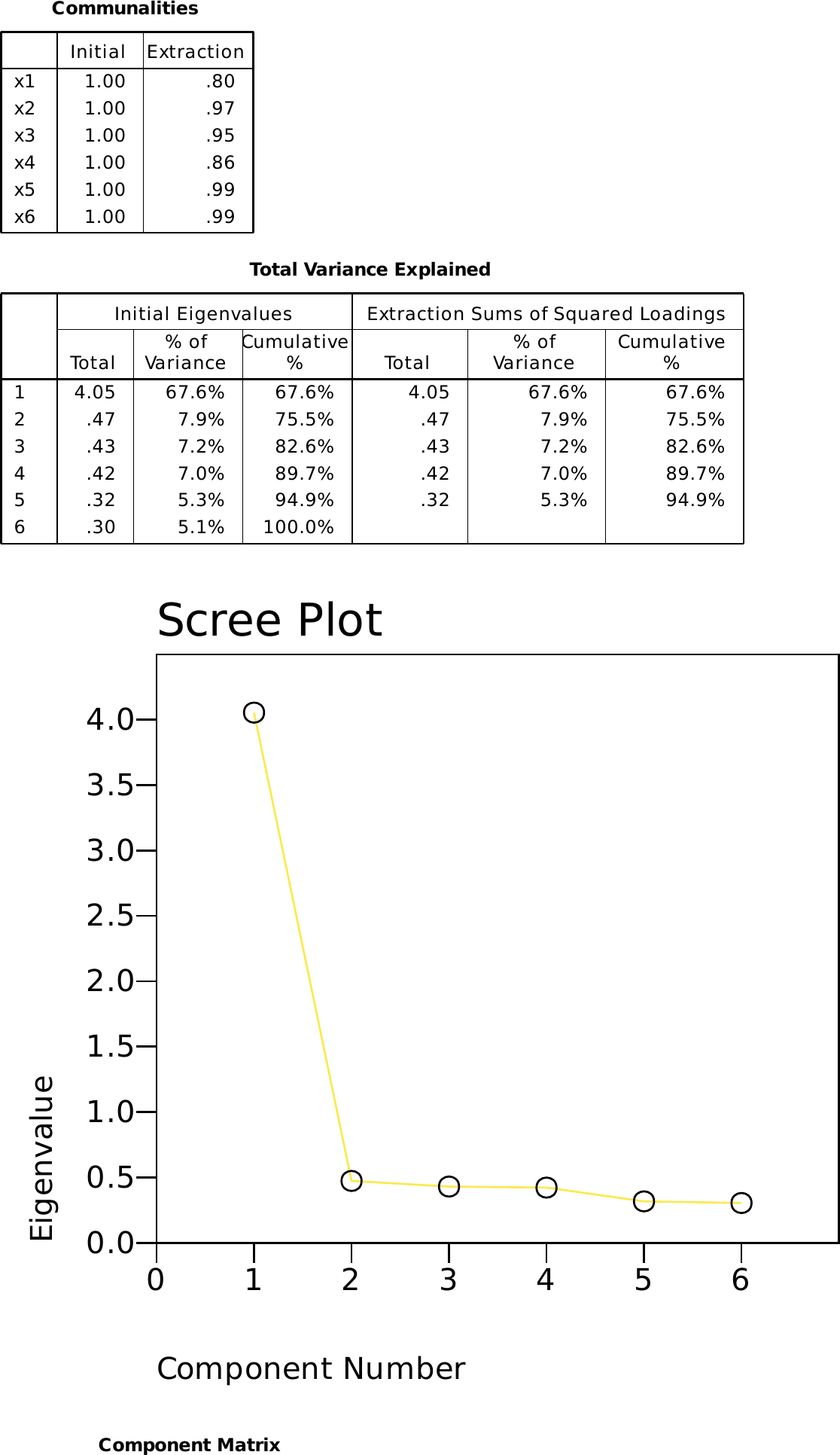
Principal Component Analysis (PCA) summarizes a set of variables by the directions along which they vary most. It is a quick dimensionality check and a collinearity remedy, not a measurement model. If one construct runs through your items, the first component should dominate:
NoteWorking in SPSS, Julia, or Python?
The code tabs below assume this chapter’s data is already loaded. Grab the one-file setup for your language from Getting the Book’s Data, run it once, then load what you need by name - this chapter uses ch19-items. For example, book_data("ch19-items") in R, Julia, or Python, or !bookdata name = "ch19-items". in SPSS. Every language reads the same shipped files, so your numbers will match the ones printed here exactly.
pc <-prcomp(items, scale. =TRUE)# eigenvalues: one large, the rest small = one dimensiontibble(component =paste0("PC", seq_along(pc$sdev)), eigenvalue = pc$sdev^2) |>round2()
One eigenvalue well above the rest is the signature of a single underlying dimension. PCA also gives the orthogonal components you can regress on when you would rather dissolve collinearity than interpret individual predictors.
Exploratory Factor Analysis (EFA) is for when you do not yet know the structure; you let the data suggest how many factors there are and which items load where. Base R’s factanal fits it by maximum likelihood:
fa1 <-factanal(items, factors =1)# all items load on the common factortibble(item =names(items), loading =as.numeric(fa1$loadings)) |>round2()
item
loading
x1
0.75
x2
0.73
x3
0.82
x4
0.80
x5
0.82
x6
0.76
INSERT FILE='data/sim/ch19-items.sps'.

* In SPSS this reads /EXTRACTION=ML, which is what the R tab's factanal()
* does. PSPP - the free engine this book renders with - offers PAF, PC and
* PA1 but not ML, so principal axis factoring is what runs here. On this data
* the two agree to the two decimals we print.
FACTOR
  /VARIABLES=x1 x2 x3 x4 x5 x6
  /EXTRACTION=PAF
  /CRITERIA=FACTORS(1)
  /PRINT=INITIAL EXTRACTION.
import pandas as pditems = pd.read_csv("data/sim/ch19-items.csv")from sklearn.decomposition import FactorAnalysisfa1 = FactorAnalysis(n_components=1).fit(items)fa1.components_.round(2) # all items load on the common factor
array([[0.98, 0.86, 1.06, 1.03, 1.12, 0.91]])
In practice you would decide the number of factors more carefully. Parallel analysis is the modern standard:
library(psych)fa.parallel(items, fa ="fa") # how many factors? compare to random datafa(items, nfactors =2, rotate ="oblimin", fm ="ml") # extract and rotate to interpret
Confirmatory Factor Analysis (CFA) is for when theory or a prior EFA has already specified the structure. You fit that structure as a fixed hypothesis to fresh data and ask whether it holds before trusting the subscale scores. This is the factor-analysis chapter’s territory; the idiom is lavaan:
library(lavaan)model <-'construct =~ x1 + x2 + x3 + x4 + x5 + x6'fit <-cfa(model, data = d)fitMeasures(fit, c("cfi", "tli", "rmsea", "srmr")) # does the one-factor model fit?
The rule that ties the three together: explore first, confirm on fresh data, and only then aggregate. PCA and EFA help you discover the structure; CFA earns you the right to treat a composite as measuring one thing.
12.5 When Not to Reduce: Reflective vs. Formative
Data reduction is powerful, but it rests on an assumption you should make on purpose. Factor analysis and SEM are built for reflective measurement: the construct is a common cause of its indicators (depression makes you sad and tired and pessimistic, so those items correlate). Averaging reflective indicators is exactly right.
Some constructs, though, are formative, or emergent: the indicators compose the construct rather than reflect it. Trust, in the authors’ own research, is better understood as a combination of good intentions, understanding, and reliability. Those three need not correlate, and a person can be high on one and low on another. Force a single reflective factor onto a formative construct and the tool becomes misleading, because it assumes the wrong causal direction. The question is not whether a latent model can fit, but whether it is the right model at all. So before you reduce, ask which kind of construct you have. Reduce reflective constructs; model formative ones as what they are.
12.6 Multiple Measures and Triangulation
A construct is something you cannot see directly. You approach it through several imperfect windows, and the strongest inference comes from triangulation: several measures that agree despite their different flaws. For social scientists this is not a luxury; it is the heart of the work, because our subject matter - purpose, curiosity, trust, anxiety - is unobservable by definition.
Two practical consequences follow. First, prefer several measures to one, and combine them (as above) into more dependable estimates. Second, before you compare two constructs, check that they are measured equally well. As the authors argue in their purpose-and-happiness work, if one of two constructs is more reliable than the other, any comparison between them is confounded by measurement quality before the substance is even in play. Vet the rulers before you trust the differences they report. For the study of the unobservable, measurement quality is not a preliminary to the science; it is the science.
12.7 What This Chapter Teaches
Reduce to gain power. Reliable composites shrink error variance, un-attenuate effects, and buy power from a sample you already have.
Check, then collapse. Confirm the items cohere (alpha), then combine them (sum, mean, or POMP); reserve factor scores for measurement work.
Test the structure first. PCA and EFA to discover it, CFA to confirm it: explore, confirm on fresh data, then aggregate.
Match the tool to the construct. Reduce reflective constructs; do not force a reflective model onto a formative one.
Triangulate. For unobservable constructs, multiple well-vetted measures are how you earn a strong inference.
12.8 Where We Go Next
With reliable, well-structured measures in hand, we are finally ready to build models with them. That is the work of the next part, where the General Linear Model takes center stage. A model is only as trustworthy as the measures feeding it, which is why this preparation came first.