Most of this book has modelled outcomes that can, in principle, go anywhere. A GPA, a reaction time, a depression score - we treat them as though the number line runs off in both directions and the only question is where the mean sits. For a great many measures that is a harmless fiction.
For others it is not, and this chapter is about those. A proportion cannot be negative. A percentage cannot exceed 100. A well-being score expressed as a percent of maximum possible is pinned at both ends by the instrument itself. When the outcome has a floor and a ceiling, a model that does not know about them will say impossible things, and it will say them with a straight face.
This matters more in this book than in most, because we have been telling you to build exactly this kind of outcome since the z-distribution chapter. POMP - \(100 \times \frac{X - \text{min}}{\text{max} - \text{min}}\) - is our house ruler for comparing measures. It is also, by construction, a bounded outcome. So we owe you the model that respects it.
20.1 Learning Objectives
See concretely how ordinary regression fails on a bounded outcome.
Model a binary outcome with logistic regression, and read the result on the probability scale.
Understand the beta distribution through its mean and precision.
Fit a beta regression to a proportion, from scratch and with a package.
Recognise the boundary problem - exact 0s and 1s - and decide about it deliberately.
NoteWorking in SPSS, Julia, or Python?
This chapter uses ch34-wellbeing. Grab the one-file setup for your language from Getting the Book’s Data, run it once, then load by name.
20.2 The Data
Two hundred and forty people in a well-being programme, half in a treatment arm and half not, with the number of weeks each has been enrolled. The outcome is a well-being questionnaire scored on its own POMP scale: 0 if you answer at the bottom of every item, 100 if you answer at the top.
INSERT FILE='data/sim/ch34-wellbeing.sps'.

* How many people sit exactly on the floor of the scale?
COMPUTE at_floor = (wellbeing = 0).
EXECUTE.
MEANS TABLES=wellbeing at_floor BY group
  /CELLS=COUNT MEAN MIN MAX.
               Case Processing Summary
+-----------------+---------------------------------+
|                 |              Cases              |
|                 +-----------+---------+-----------+
|                 |  Included | Excluded|   Total   |
|                 +---+-------+-+-------+---+-------+
|                 | N |Percent|N|Percent| N |Percent|
+-----------------+---+-------+-+-------+---+-------+
|wellbeing * group|240| 100.0%|0|    .0%|240| 100.0%|
|at_floor * group |240| 100.0%|0|    .0%|240| 100.0%|
+-----------------+---+-------+-+-------+---+-------+

    wellbeing * at_floor * group
+---------------+---------+--------+
|group          |wellbeing|at_floor|
+---------------+---------+--------+
|control N      |      120|     120|
|        Mean   |27.421258|     .11|
|        Minimum|  .000000|     .00|
|        Maximum|67.230200|    1.00|
+---------------+---------+--------+
|treated N      |      120|     120|
|        Mean   |45.370979|     .03|
|        Minimum|  .000000|     .00|
|        Maximum|86.305900|    1.00|
+---------------+---------+--------+
|Total   N      |      240|     240|
|        Mean   |36.396119|     .07|
|        Minimum|  .000000|     .00|
|        Maximum|86.305900|    1.00|
+---------------+---------+--------+
           n  at_floor  lowest  highest
group
control  120        13     0.0  67.2302
treated  120         4     0.0  86.3059
Seventeen people scored exactly zero. That is not a rounding artefact and it is not missing data. They answered at the bottom of every item, which is a thing the instrument allows, so zero is their score. Hold on to those seventeen; they turn out to be the most interesting people in the dataset.
20.3 What Ordinary Regression Says
Start with the model we would reach for out of habit: well-being on group, fitted by least squares.
# What does it predict for a control participant, with 95% prediction interval?predict(ols, tibble(group =factor("control", levels =levels(d$group))),interval ="prediction") |>as_tibble() |># predict() hands back a matrix; round2() wants a frameround2()
fit
lwr
upr
27.42
-6.89
61.73
INSERT FILE='data/sim/ch34-wellbeing.sps'.

* Least squares on a bounded outcome. Watch the residual spread by group,
* and note that nothing in this model knows the scale stops at 0 and 100.
COMPUTE treated = (group = 'treated').
EXECUTE.

REGRESSION
  /STATISTICS=COEFF R ANOVA
  /DEPENDENT wellbeing
  /METHOD=ENTER treated
  /SAVE PRED RESID.
                 Model Summary (wellbeing)
+---+--------+-----------------+--------------------------+
| R |R Square|Adjusted R Square|Std. Error of the Estimate|
+---+--------+-----------------+--------------------------+
|.46|     .21|              .21|                     17.34|
+---+--------+-----------------+--------------------------+

                   ANOVA (wellbeing)
+----------+--------------+---+-----------+-----+----+
|          |Sum of Squares| df|Mean Square|  F  |Sig.|
+----------+--------------+---+-----------+-----+----+
|Regression|      19331.55|  1|   19331.55|64.26|.000|
|Residual  |      71595.69|238|     300.82|     |    |
|Total     |      90927.24|239|           |     |    |
+----------+--------------+---+-----------+-----+----+

                           Coefficients (wellbeing)
+----------+----------------------------+-------------------------+-----+----+
|          | Unstandardized Coefficients|Standardized Coefficients|     |    |
|          +-----------+----------------+-------------------------+     |    |
|          |     B     |   Std. Error   |           Beta          |  t  |Sig.|
+----------+-----------+----------------+-------------------------+-----+----+
|(Constant)|      27.42|            1.58|                      .00|17.32|.000|
|treated   |      17.95|            2.24|                      .46| 8.02|.000|
+----------+-----------+----------------+-------------------------+-----+----+
usingCSV, DataFrames, GLMd = CSV.read("data/sim/ch34-wellbeing.csv", DataFrame)d.treated =Float64.(d.group .=="treated")ols =lm(@formula(wellbeing ~ treated), d)# show(..., MIME) prints the coefficient table. Echoing the model object# itself dumps its Julia type, which tells a reader nothing.show(stdout, MIME("text/plain"), coeftable(ols))
The coefficients look reasonable. The prediction interval does not. Its lower bound is about -6.9 - a negative percent of maximum possible, which is not a number the instrument can produce. The model is telling us, in perfectly good faith, that a plausible score is one that cannot exist.
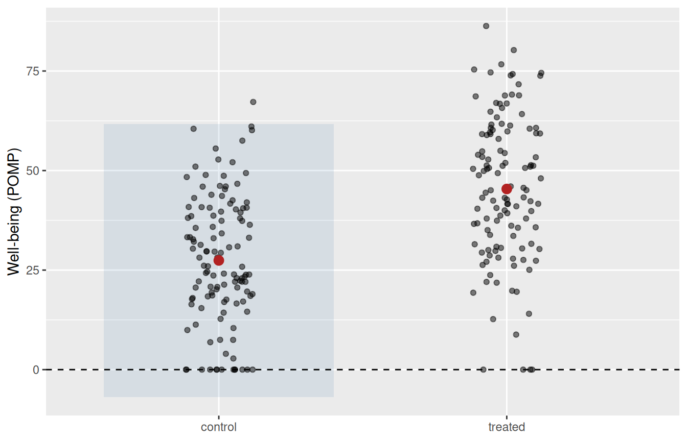
That is the first failure and the easiest to see. The second is quieter. Least squares assumes the spread of the residuals is the same everywhere, and on a bounded scale it cannot be: near a boundary there is simply less room to vary. Look at the two arms together with their fitted values.
Well-being by arm on the POMP scale. The dashed line is the floor of the instrument; the shaded band is where ordinary regression thinks a control participant might plausibly score. Part of it lies below a score that can exist.
The pile-up along the dashed line is the seventeen. No symmetric, constant-variance model can put them there.
20.4 Two Kinds of Bounded Outcome
Before the fix, a distinction worth getting right, because these two get run together constantly and they are not the same thing.
A binary outcome is one event: did this person reach the halfway mark, yes or no. It is 0 or 1 and nothing between. The natural model is logistic regression, and its coefficients really are log odds, built from counts of successes and failures.
A proportion is a continuous quantity between 0 and 1: what fraction of the possible score did this person reach. It can be 0.37. There are no successes and failures to count. The natural model is beta regression.
Both are bounded, and both use a logit link to keep the fitted values inside the boundary. That shared machinery is why they are confused. But the logit means different things in the two models, and a table is the clearest way to hold them apart.
Binary
Proportion
The outcome is
0 or 1
any value in (0, 1)
Example here
reached POMP 50?
POMP score / 100
Distribution
Bernoulli / binomial
beta
Model
logistic regression
beta regression
The logit is
genuinely log odds
a map from the mean onto the real line
Exponentiated coefficient
an odds ratio
not an odds ratio
That last row is the one that bites. In a beta regression you can still exponentiate a coefficient, and R will happily print the number, but it is not an odds ratio because there are no odds - no successes, no failures, nothing being counted. The logit is doing a humbler job there: taking a mean that has to live between 0 and 1 and stretching it onto a scale where a straight line is a sensible thing to fit.
20.5 Binary: Logistic Regression
Take the simple question first. Did each person reach the halfway mark of the scale?
d <- d |>mutate(reached50 =as.integer(wellbeing >=50))fit_bin <-glm(reached50 ~ group, family = binomial, data = d)tidy2(fit_bin)
term
estimate
std.error
statistic
p.value
(Intercept)
-2.51
0.35
-7.25
< .001
grouptreated
2.28
0.39
5.81
< .001
# On the probability scale, which is where people actually thinktibble(group =factor(c("control", "treated"), levels =levels(d$group))) |>mutate(p_reach50 =predict(fit_bin, pick(everything()), type ="response")) |>round2()
group
p_reach50
control
0.08
treated
0.44
INSERT FILE='data/sim/ch34-wellbeing.sps'.

* Binary outcome: did the person reach the halfway mark of the scale?
COMPUTE reached50 = (wellbeing >= 50).
COMPUTE treated   = (group = 'treated').
EXECUTE.

LOGISTIC REGRESSION reached50 WITH treated.
  Dependent Variable Encoding
+--------------+--------------+
|Original Value|Internal Value|
+--------------+--------------+
|.00           |           .00|
|1.00          |          1.00|
+--------------+--------------+

      Case Processing Summary
+--------------------+---+-------+
|Unweighted Cases    | N |Percent|
+--------------------+---+-------+
|Included in Analysis|240| 100.0%|
|Missing Cases       |  0|    .0%|
|Total               |240| 100.0%|
+--------------------+---+-------+

note: Estimation terminated at iteration number 5 because parameter estimates
changed by less than 0.001

                          Model Summary
+----+-----------------+--------------------+-------------------+
|Step|-2 Log likelihood|Cox & Snell R Square|Nagelkerke R Square|
+----+-----------------+--------------------+-------------------+
|1   |           228.65|                 .17|                .25|
+----+-----------------+--------------------+-------------------+

                   Classification Table
+--------------------------+-----------------------------+
|                          |          Predicted          |
|                          +----------+------------------+
|                          | reached50|                  |
|                          +----+-----+                  |
|       Observed           | .00| 1.00|Percentage Correct|
+--------------------------+----+-----+------------------+
|Step 1 reached50   .00    | 178|    0|            100.0%|
|                   1.00   |  62|    0|               .0%|
|      --------------------+----+-----+------------------+
|       Overall Percentage |    |     |             74.2%|
+--------------------------+----+-----+------------------+

            Variables in the Equation
+---------------+-----+----+-----+--+----+------+
|               |  B  |S.E.| Wald|df|Sig.|Exp(B)|
+---------------+-----+----+-----+--+----+------+
|Step 1 treated | 2.28| .39|33.71| 1|.000|  9.76|
|       Constant|-2.51| .35|52.54| 1|.000|   .08|
+---------------+-----+----+-----+--+----+------+
Nine of 120 control participants reached the halfway mark; 53 of 120 in the treatment arm did. On the probability scale that is 0.08 against 0.44. The coefficient for treated is 2.28 on the log-odds scale, and exponentiating gives an odds ratio of about 9.8 - here that genuinely is an odds ratio, because we counted successes and failures to get it.
ImportantReport the probability, not the log odds
A coefficient of 2.28 means nothing to a reader, and an odds ratio of 9.8 means less than most people think - odds ratios are not risk ratios, and they diverge badly when the outcome is common. The number a reader can act on is the pair of probabilities: 8% against 44%. Fit on the logit scale because that is where the model is linear; report on the probability scale because that is where your audience lives.
20.6 The Beta Distribution
Now the harder and more useful case: the POMP score itself, as a proportion between 0 and 1.
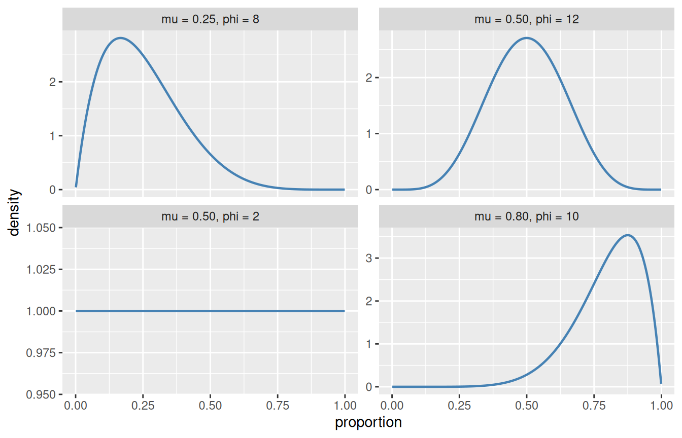
We need a distribution that lives on that interval and can take a variety of shapes - piled near the floor, piled near the ceiling, humped in the middle, or spread flat. The beta distribution does all of that with two parameters.
It is usually written with two shape parameters, \(a\) and \(b\), but that pair is hard to think with. For regression there is a much friendlier parameterisation in terms of a mean\(\mu\) and a precision\(\phi\):
Read that variance formula slowly, because it contains the whole point of the chapter. The variance is not a free parameter. It is determined by the mean. As \(\mu\) approaches 0 or 1, \(\mu(1-\mu)\) shrinks toward zero and so does the variance. The distribution automatically has less room to vary near the boundaries - which is exactly the behaviour we saw in the data and exactly what least squares assumes away.
The precision \(\phi\) controls how tightly the distribution concentrates around its mean: larger \(\phi\), narrower spread.
Four beta distributions, all written as a mean and a precision. The same two numbers produce a floor-heavy shape, a symmetric hump, a ceiling-heavy shape, and a nearly flat one.
20.7 Beta Regression, By Hand
A beta regression says: each person’s proportion is a draw from a beta distribution whose mean depends on their predictors through a logit link, with a precision \(\phi\) shared across everyone.
That is the entire model, and it is short enough to fit from scratch. We write down the negative log-likelihood and hand it to an optimiser - the same move the Rasch chapter makes for JMLE and the latent class chapter makes for EM.
One thing has to be dealt with first. The beta density is zero at exactly 0 and exactly 1, so the log-likelihood of our seventeen floor-sitters is \(-\infty\). The standard move is to squeeze the scale very slightly inward, so that 0 becomes a small positive number instead:
\[y' = \frac{y(n-1) + 0.5}{n}\]
We will come back to whether that is a good idea. For now, notice that it is a decision, and that we are making it in the open.
n <-nrow(d)d <- d |>mutate(p = wellbeing /100, # POMP as a proportionpy = (p * (n -1) +0.5) / n) # squeezed off the boundaryX <-model.matrix(~ group, d)k <-ncol(X)# Negative log-likelihood: mean through a logit link, one shared precision.# phi is fitted on the log scale so the optimiser cannot wander negative.nll <-function(par) { mu <-plogis(X %*% par[1:k]) phi <-exp(par[k +1])-sum(dbeta(d$py, mu * phi, (1- mu) * phi, log =TRUE))}fit <-optim(c(0, 0, log(5)), nll, method ="BFGS", hessian =TRUE)tibble(term =c(colnames(X), "log(phi)"),estimate = fit$par,std.error =sqrt(diag(solve(fit$hessian)))) |>round2()
term
estimate
std.error
(Intercept)
-1.08
0.09
grouptreated
0.82
0.12
log(phi)
1.38
0.08
* Base SPSS has no beta regression. GENLIN offers binomial, Poisson, gamma
* and several other families, but not beta, and there is no user-written
* equivalent that ships with it.
*
* Where it does exist:
*   R      betareg::betareg(y ~ x)
*   Stata  betareg y x          (built in)
*   Python statsmodels.othermod.betareg.BetaModel
*
* The nearest honest thing base SPSS can do is the logistic model above, on
* a binary version of the outcome, which answers a different question and
* discards the difference between a score of 51 and a score of 99.
usingCSV, DataFrames, Distributions, Optimd = CSV.read("data/sim/ch34-wellbeing.csv", DataFrame)n =nrow(d)p = d.wellbeing ./100py = (p .* (n -1) .+0.5) ./ nX =hcat(ones(n), Float64.(d.group .=="treated"))logistic(x) =1/ (1+exp(-x))functionnll(par)# Clamp the fitted mean off 0 and 1. The optimiser will try values that# round to exactly 1, and Beta() rejects a zero shape parameter outright. mu =clamp.(logistic.(X * par[1:2]), 1e-9, 1-1e-9) phi =exp(par[3])-sum(logpdf.(Beta.(mu .* phi, (1.- mu) .* phi), py))endres =optimize(nll, [0.0, 0.0, log(5.0)], BFGS())round.(Optim.minimizer(res), digits =4)
library(betareg)fit_beta <-betareg(py ~ group, data = d)tidy2(fit_beta)
component
term
estimate
std.error
statistic
p.value
mean
(Intercept)
-1.08
0.09
-12.21
< .001
mean
grouptreated
0.82
0.12
6.90
< .001
precision
(phi)
3.98
0.34
11.86
< .001
* Still no beta family in base SPSS - see the note in the tab above.
* The R, Julia, and Python tabs fit the model; this one cannot.
# No maintained beta-regression package is loaded in this book's Julia# environment, so the hand-written likelihood above IS the fit. GLM.jl# covers the exponential family - binomial, Poisson, gamma - but the beta# is not a member of it in the form GLM.jl uses.
The hand-written optimiser and betareg agree to four decimal places on every coefficient and on \(\phi\). That is worth pausing on: the package is not doing anything mysterious. It is writing down the same likelihood and handing it to the same kind of optimiser, with better error handling and a nicer print method. Now that you have seen the fifteen lines, betareg is a convenience rather than an oracle.
20.8 Reading the Answer
Coefficients from a beta regression are on the logit scale, which is not where anyone thinks. Convert them back.
fit_full <-betareg(py ~ group + weeks, data = d)tidy2(fit_full)
component
term
estimate
std.error
statistic
p.value
mean
(Intercept)
-1.38
0.13
-10.71
< .001
mean
grouptreated
0.84
0.12
7.15
< .001
mean
weeks
0.05
0.02
3.09
0.002
precision
(phi)
4.15
0.35
11.81
< .001
# Fitted POMP score for someone six weeks in, by armtibble(group =factor(c("control", "treated"), levels =levels(d$group)),weeks =6) |>mutate(fitted_POMP =100*predict(fit_full, pick(everything()))) |>round2()
group
weeks
fitted_POMP
control
6
25.42
treated
6
44.15
* No beta family in base SPSS; see above.
# The hand-written fit extends the same way: add a column to X for weeks# and a third coefficient to the starting vector.
Six weeks in, the model puts a control participant at about 25 on the POMP scale and a treated participant at about 44. That is the sentence to put in a paper. The coefficient of 0.84 that produced it is not.
Notice also what the model does not do: it never predicts a negative score, and it never predicts one above 100, because the logit link makes those outcomes unreachable by construction rather than unlikely by assumption.
20.9 The Boundary Problem
Now back to the seventeen, and to the quiet decision we made on their behalf.
The beta distribution is defined on the open interval - 0 and 1 are excluded. The floor-sitters are therefore not just awkward, they are outside the model’s support. We squeezed them inward with \((y(n-1)+0.5)/n\) and carried on. That is the conventional fix and it is what most published beta regressions do.
It also changes the answer, and the size of the change is not obvious. Compare three defensible choices on the same data.
compare <-bind_rows(tibble(handling ="squeezed off the boundary",tidy(betareg(py ~ group, data = d))),tibble(handling ="floor-sitters dropped",tidy(betareg(I(wellbeing /100) ~ group, data =filter(d, wellbeing >0)))),tibble(handling ="raw, zeros left in",tidy(betareg(I(wellbeing /100) ~ group, data = d)))) |>filter(term =="grouptreated") |>select(handling, estimate, std.error)compare |>round2()
handling
estimate
std.error
squeezed off the boundary
0.82
0.12
floor-sitters dropped
0.68
0.09
raw, zeros left in
0.52
0.08
Three answers, same data, same question. And the third one is the one to look at hardest.
ImportantA package answered a question that has no answer
Fitting beta regression to the raw data - zeros and all - should be impossible. The beta density is zero at the boundary, so the log-likelihood of those seventeen observations is \(-\infty\), and there is no maximum to find.
betareg() fits it anyway. It reports using all 240 rows and returns a finite log-likelihood, and if you did not already know about the boundary you would have no reason to doubt it. Computing the beta log-likelihood by hand at the model’s own fitted values, over the same 240 rows, gives -Inf.
The estimates are not a rounding difference from the honest ones either. They move the treatment effect by enough to change what you would write in a paper.
The lesson is not that betareg is bad software - it is careful, well-documented software. The lesson is that the boundary is your decision and you should make it out loud. A package cannot make it for you, but it can appear to.
So what should you do with the seventeen?
The squeeze is fine for a sensitivity check and poor as a primary analysis, because its effect depends on \(n\) - the nudge is \(1/2n\), so it shrinks as the sample grows, and the estimates drift with sample size for reasons that have nothing to do with well-being. Dropping the floor-sitters is worse than it looks: they are not a nuisance, they are the people the programme most needs to help, and throwing them out biases exactly the comparison you care about.
The principled answers keep them and model why they are there:
Zero-inflated beta treats the floor as a separate process - one model for whether someone is at the floor, another for where they are if they are not.
Zero-one-inflated beta does the same at both ends.
Ordered beta treats the floor and ceiling as ordered categories either side of the continuous middle, which needs only one set of coefficients rather than two.
All three need more machinery than this book carries - in R they live in brms and ordbetareg, which fit by Markov chain Monte Carlo through Stan. The Bayesian section gives you the ideas those rest on. What we want you to leave with is narrower and more useful: look at your outcome’s boundaries before you model it, count how many observations are sitting on them, and choose deliberately.
20.10 Challenge
TipDo One Yourself
Refit the beta regression with the squeeze constant changed from 0.5 to 0.1 and to 0.9. How much does the treatment coefficient move? Now double the sample size by simulating more data and repeat. What does the drift tell you about using the squeeze as a primary analysis?
Take any POMP-scaled outcome from your own work and count the exact 0s and 100s. If there are none, has something already been done to the data?
Fit the logistic model from this chapter with the cut at 30 and again at 70 instead of 50. Compare the three odds ratios. What has dichotomising cost you that the beta regression kept?
20.11 Where We Go Next
A bounded outcome is one case of a general idea: the distribution you assume should be one the data could actually have come from. We have now done that for proportions here and for counts nowhere - Poisson and negative binomial regression are the next step along the same road, and they belong to the same family of models reached through a link function.
The wider lesson travels further than any of them. Before choosing a model, ask what values the outcome is capable of taking. If the answer has a floor, a ceiling, or both, a model that does not know it will eventually tell you something impossible - and it will not warn you when it does.